
Ferromagnetic Dynamics - Markdown
We start by working out the equations of motion for a single ferromagnetic moment. When a magnetic moment is exposed to an external magnetic field, a torque will be present. This torque \(\mathbf{\tau}\) is given by the following equation:
\begin{equation} \mathbf{\tau} = \mathbf{m} \times \mu_{0}\mathbf{H}_{\mathrm{eff}} \end{equation}
where \(\mathbf{m}\) is the magnetic moment, \(\mu_{0}\) is the magnetic permeability of free space and \(\mathbf{H}_{\mathrm{eff}}\) is the effective field that encapsulates all the combination of external and internal fields:
\[\mathbf{H}_{\mathrm{eff}} = \mathbf{H}_{\mathrm{external}} + \mathbf{H}_{\mathrm{exchange}} + \mathbf{H}_{\mathrm{ani}} + \mathbf{H}_{\mathrm{DMI}} + ...\]where \(\mathbf{H}_{\mathrm{external}}\) is the applied magnetic field, \(\mathbf{H}_{\mathrm{exchange}}\) is the exchange field.
The associated angular momentum with this moment is given by the gyromagnetic ratio (\(\gamma\)) relation:
\begin{equation} \mathbf{m} = \gamma\mathbf{L} \end{equation}
where \(\gamma = g\mu_{B}/\hbar\), g is the Land'e g-factor, \(\mu_{B}\) is the Bohr magnetron and \(\hbar\) is the reduced Plank constant. Newton’s second law says the torque on a system equals to change in its angular momentum:
\begin{equation} \tau = \dfrac{d\mathbf{L}}{dt} = \mathbf{m} \times \mu_{0}\mathbf{H}_{\mathrm{eff}} \label{eq:angular momentum and torque} \end{equation}
And if we use the gyromagnetic ratio relation to substitute angular momentum \(\mathbf{L}\), equation can be rewritten as:
\begin{equation} \dfrac{d\mathbf{m}}{dt} = \gamma \mu_{0} (\mathbf{m} \times \mathbf{H}_{\mathrm{eff}}), \label{eq:LL Equation} \end{equation}
This equation is known as Landau-Lifshitz equation and describes the uniform precession of a magnetic moment around the applied field with the Larmor frequency \(\omega = \gamma \mu_{0} H\). This is analogous of precession of a spinning top inside a uniform gravitational field without any frictional loss.
Dissipation
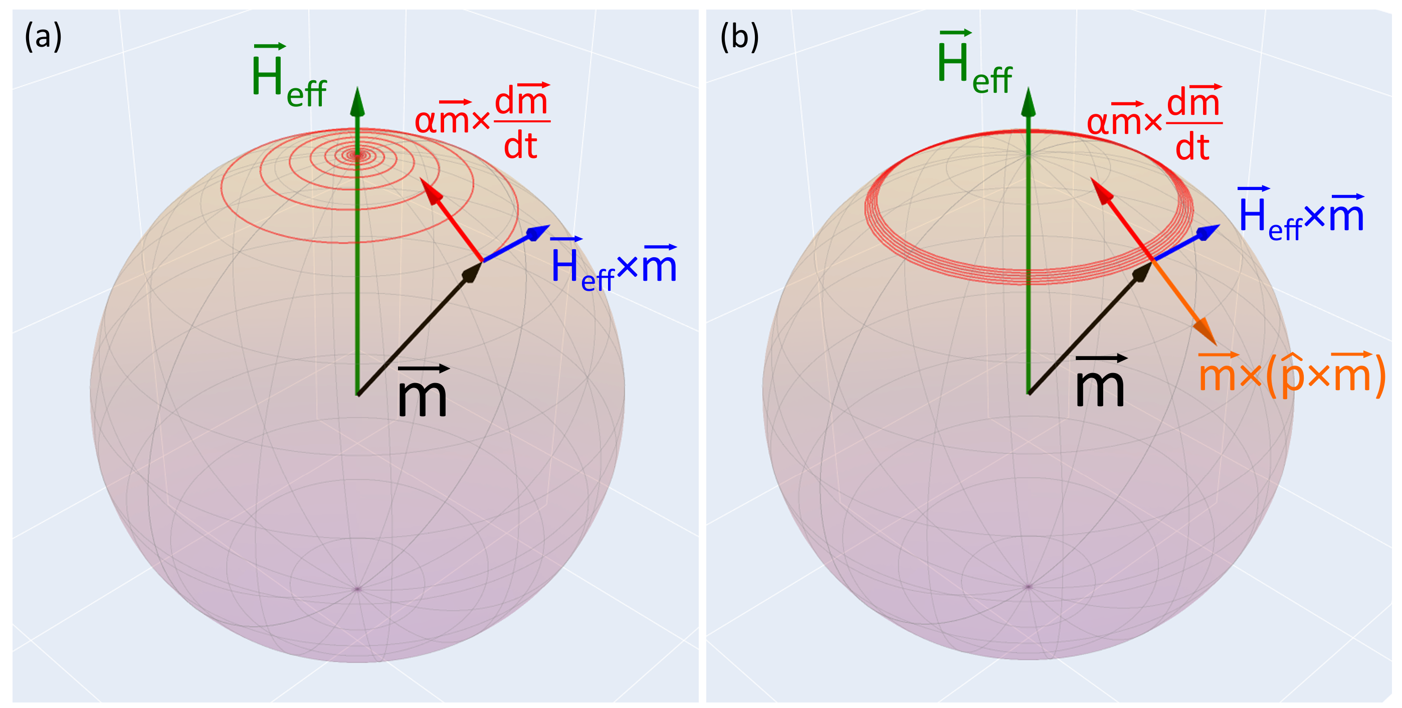
In reality, every physical system loses energy over time due to dissipational forces. To capture this Landau and Lifshitz proposed a damping term proportional to \(\mathbf{m} \times (\mathbf{m} \times \mathbf{H}_{\textrm{eff}})\), which is always perpendicular to the orbit, so that precession slowly dies out. Later, Gilbert modified the damping term into \(\alpha m \times \dfrac{d\mathbf{m}}{dt}\) and the resulting equation is now known as Landau-Lifshitz-Gilbert (LLG) equation:
\[\dfrac{d\mathbf{m}}{dt} = \gamma \mu_{0} (\mathbf{m} \times \mathbf{H}_{\mathrm{eff}} )+ \alpha (\mathbf{m} \times \frac{d\mathbf{m}}{dt} )\]where \(\alpha\) is the dimensionless Gilbert damping parameter. It is a phenomenological constant that encompasses multiple methods of dissipation of angular momentum from spin precession to the lattice. The methods include dissipation via spin-orbit coupling, scattering processes and non-local spin relaxation processes.
An interesting aspect of the Gilbert damping term is that it is proportional to the change of magnetization \(\frac{d\mathbf{m}}{dt}\), meaning an increase in the rotation rate of magnetization increases the damping of the system.
Spin (Transfer) Torques
In 1996, Slonczewski and Berger independently realized that the effects of Gilbert damping can be countered by spin-transfer torques and lead to magnetization switching or stable oscillations in spin valves. They expanded LLG the model to account for the spin-transfer torque term. This equation is now known as Landau-Liftshitz-Gilbert-Slonczewski (LLGS) equation:
\[\begin{equation} \frac{d\mathbf{m}}{dt} = \gamma \mathbf{H}_{\textrm{eff}}\times\mathbf{m} +\alpha\mathbf{m}\times\frac{d\mathbf{m}}{dt} + \tau_{ST} \end{equation}\]where \(H_{\textrm{eff}}\) is the effective magnetic field, \(\gamma\) is the gyromagnetic ratio, \(\alpha\) is the Gilbert damping constant and \(\tau_{ST}\) is the spin torque. Again this torque can be decomposed into field-like and damping-like components:
\begin{equation} \mathbf{\tau} = \tau_{\textrm{DL}} \mathbf{m} \times (\mathbf{p} \times \mathbf{m}) + \tau_{\textrm{FL}} \mathbf{m} \times \mathbf{p} \end{equation}
where \(\mathbf{p}\) is the polarization vector usually set by the symmetry of the system, \(\tau_{\textrm{DL}}\) and \(\tau_{\textrm{FL}}\) are field-like and damping-like torques respectively. It is again beneficial to decompose the torques like this because damping-like torques (\(\tau_{\textrm{DL}}\)) and field-like torques (\(\tau_{\textrm{FL}}\)) affect the magnetization in fundamentally different ways. Damping-like torques change the energy of the system and can switch the magnetization, whereas field-like torques act like an effective field and only change the precession frequency.
For the antiferromagnetic case, LLGS equation above becomes two coupled equation one for each sublattice:
\[\frac{d\mathbf{m}_1}{dt} = \gamma \mathbf{H}_1^{\textrm{eff}}\times\mathbf{m}_1 +\alpha\mathbf{m}_1\times\frac{d\mathbf{m}_1}{dt} + \tau_1^{FL} + \tau_1^{DL} \nonumber\] \[\frac{d\mathbf{m}_2}{dt} = \gamma \mathbf{H}_2^{\textrm{eff}}\times\mathbf{m}_2 +\alpha\mathbf{m}_2\times\frac{d\mathbf{m}_2}{dt} + \tau_2^{FL} + \tau_2^{DL}\]where the coupling is associated the exchange interaction is included in the effective field term, \(\mathbf{H}_{1,2}^{\textrm{eff}}\).