Bootstrapping for Confidence Intervals and A/B testing

When running experiments, like A/B tests, understanding uncertainty and statistical significance is extremely crucial. This post explores how the bootstrapping method helps to calculate confidence intervals and p-values in an A/B test scenario.

The two main questions that we are trying to answer are:

1. How do we calculate the confidence interval for the metric we are measuring?
2. How do we determine if the results of an A/B test are statistically significant?

Scenario: A/B Test on Sign-Up Button Color

Imagine you’re a data scientist testing a new design for a website’s sign-up button. The original button is blue, and you’re testing an orange version, hypothesizing that it will lead to higher sign-up rates.

To correctly evaluate the experiment, we need to:

• Measure the current sign-up rate (control group).
• Compare it to the sign-up rate with the new button (experiment group).
• Account for uncertainty in these measurements.

What is Bootstrapping?

Bootstrapping is a resampling method that involves generating multiple “fake” datasets by randomly sampling (with replacement) from the observed data. Each sample provides a slightly different perspective on the underlying distribution, enabling us to estimate the uncertainty of our metrics.

Resampling with replacement ensures variability, mimicking our uncertainty about the population. Additionally, Central Limit Theorem helps ensure that the means of our resampled datasets follow a normal distribution.

We use bootstrapping to: (1) Compute confidence intervals. (2) Conduct hypothesis testing.

Calculating Confidence Intervals

To understand the uncertainty in our measurements, we calculate confidence intervals for the observed sign-up rate in the control group. Bootstrapping allows us to estimate these intervals without relying on theoretical assumptions about the underlying distribution.

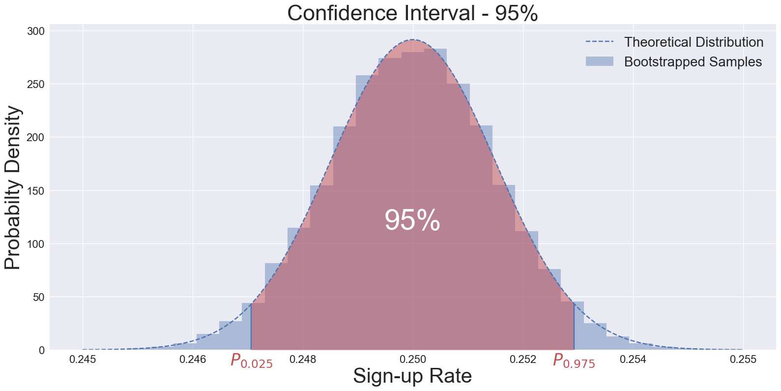Fig. 1: A histogram showing distribution of means of 50,000 bootstrapped samples. Original (measured) data set has 10,000 visitors with 25% sign-up rate.

Steps:

1. Resample the observed data multiple times (e.g., 50,000 iterations).
2. Compute the metric of interest (e.g., mean sign-up rate) for each resampled dataset.
3. Sort the metric values and extract the desired percentiles (e.g., 2.5th and 97.5th for a 95% confidence interval).

Code:

# Calculate 95% confidence intervals using bootstrapping
ctrl_bootstrap_means = []
for i in range(50_000):
    ctrl_bootstrap_means.append(
        np.random.choice(ctrl_dataset,len(ctrl_dataset),replace=True).mean()
        )

lower_bound = np.percentile(ctrl_bootstrap_means, 2.5)
upper_bound = np.percentile(ctrl_bootstrap_means, 97.5)
print(f"95% CI for bootstrapped samples: {lower_bound:.5f}, {upper_bound:.5f}")

Output:

95% CI for bootstrapped samples: 0.24730, 0.25269

Hypothesis Testing with Bootstrapping

In an A/B test, the goal is to evaluate whether the experimental group (orange button) performs significantly better than the control group (blue button). Bootstrapping provides a way to calculate p-values by resampling.

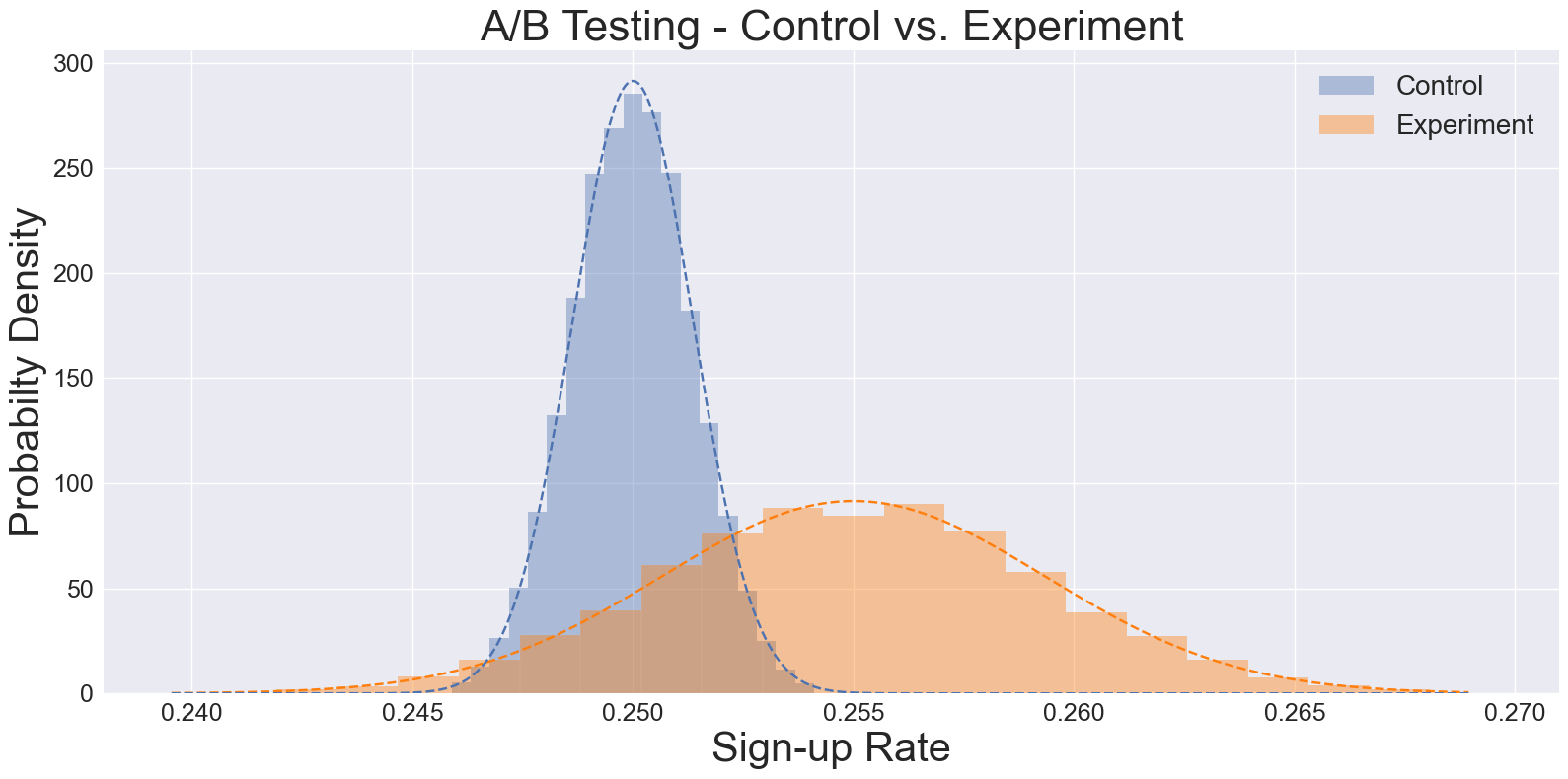Fig 2: A histogram showing bootstrapped samples from control and experiment group.

Steps:

1. Resample both control and experimental groups (e.g., 50,000 iterations each).
2. Record the mean sign-up rate for each resampled dataset.
3. Compute the difference between the bootstrapped means.
4. Estimate the p-value as the proportion of iterations where the experimental group performed worse than or equal to the control group. Code:

# Bootstrapping for hypothesis testing
diff_means = []
for i in range(50_000):
    diff_means.append(
        np.random.choice(exp_dataset, len(exp_dataset), replace=True).mean() 
        - np.random.choice(ctrl_dataset, len(ctrl_dataset), replace=True).mean()
    )
        
p_value = (np.array(diff_means) <= 0).mean()
print(f"P-value: {p_value:.5f}")

Output:

P-value: 0.13634

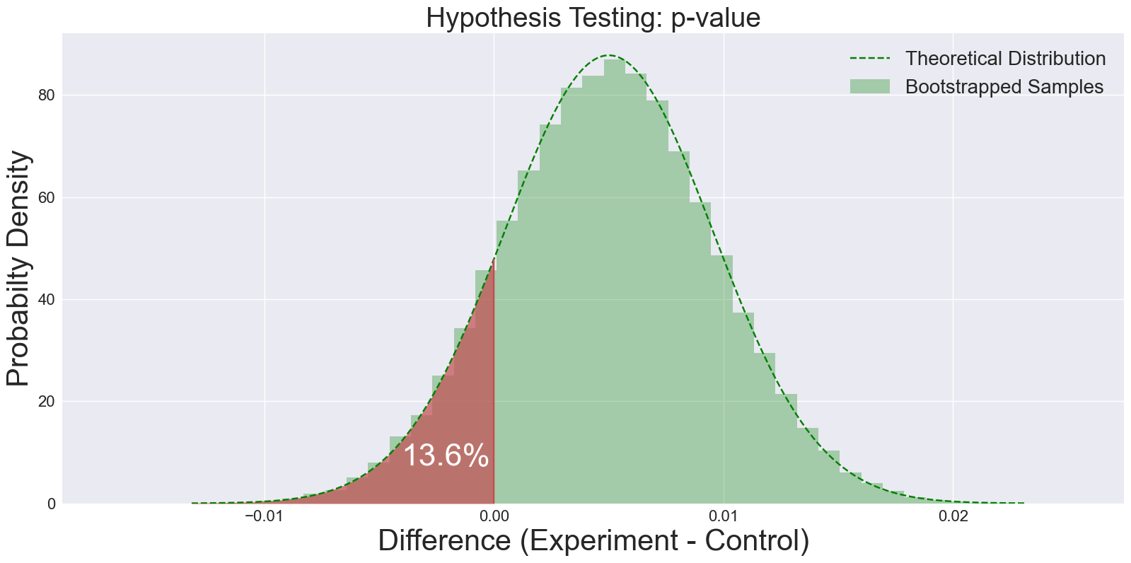Fig 3: A histogram of the differences of bootstrapped samples. Proportion of values below zero represents the p-value.

A p-value of 0.136 is significantly higher than the traditionally chosen 0.05 limit. That means under the null hypothesis (e.g. if there is no difference between experiment and control), there is 13.6% chance of seeing a result like this just due to random chance. Therefore we can’t reject the null hypothesis!

Comparing Bootstrap Results to Theoretical Values

Bootstrapping is particularly valuable when:

• The sample size is small.
• The data does not follow standard distributions (e.g., normal or binomial).

However, when assumptions about the distribution hold (e.g., binomial for success/failure data), theoretical calculations can serve as a benchmark. Let’s compare our findings to theoretical values:

1. Confidence intervals derived from bootstrapping vs. theoretical methods:

Compare this to the theoretical confidence interval derived using a binomial distribution:

The confidence interval for a binomial distribution can be calculated from:

\begin{equation} CI = \hat{p} \pm Z_{\alpha/2} \cdot \sqrt{\frac{\hat{p}(1 - \hat{p})}{n}} \end{equation}

Where:

• \(\hat{p}\) = observed proportion (e.g., success rate)
• \(Z_{\alpha/2}\) = Z-score corresponding to the desired confidence level / p-value
• \(n\) = sample size

# Calculate 95% confidence intervals using theoretical distribution
ctrl_std_err = np.sqrt(ctrl_mean * (1 - ctrl_mean) / len(ctrl_dataset))
ci_lower = ctrl_mean - sp.stats.norm.ppf(0.975) * ctrl_std_err
ci_upper = ctrl_mean + sp.stats.norm.ppf(0.975) * ctrl_std_err
print(f"95% CI from theoretical binomial distribution: {ci_lower:.5f}, {upper_bound:.5f}")

Output:

95% CI from theoretical binomial distribution: 0.24732, 0.25269

2. P-values obtained from bootstrapping vs. traditional hypothesis tests:

The test statistic for hypothesis testing of the difference between two proportions is given by:

Where:

• \(\hat{p}_A\) = observed proportion for group A
• \(\hat{p}_B\) = observed proportion for group B
• \(\hat{p} = \frac{x_A + x_B}{n_A + n_B}\) = pooled proportion across both groups
• \(n_A, n_B\) = sample sizes for groups A and B
• \(x_A, x_B\) = number of successes for groups A and B

# Calculate pooled proportion under the null hypothesis
pooled_successes = np.sum(ctrl_dataset) + np.sum(exp_dataset)
pooled_trials = len(ctrl_dataset) + len(exp_dataset)
pooled_proportion = pooled_successes / pooled_trials

# Combined standard error
se_combined = np.sqrt(
    pooled_proportion * (1 - pooled_proportion) * (1 / len(ctrl_dataset) + 1 / len(exp_dataset)))

# Z-test statistic
z_stat = (exp_mean - ctrl_mean) / se_combined

# P-value for one-tailed test
p_value =  (1 - sp.stats.norm.cdf(abs(z_stat)))

# Output results
print(f"Z-Statistic: {z_stat:.4f}")
print(f"P-Value: {p_value:.4f}")

Output:

Z-Statistic: 1.10030
P-Value: 0.13560

In all cases, bootsrapped calculation and theory match at least 3^rd digits after decimal!

Key Considerations for Bootstrapping:

The sampled data must be unbiased. Bootstrapping assumes the observed data represents the population well.

Conclusion

Bootstrapping is my go-to tool for estimating uncertainty and testing hypotheses, particularly when I am presenting to non-technical stakeholders. Through this method, you can:

• Understand (and visualize) the range of plausible values for your metrics.
• Test hypotheses with fewer assumptions, leveraging the power of resampling.
• Develop a more intuitive understanding of confidence intervals and hypothesis testing!